In this blog post, I will explain some of the technical details behind my implementation of a deferred PBR renderer in OpenGL.
I won’t go into too many details about the computer graphics concepts applied here. If that’s something of interest to you, you can read LearnOpenGL which is where I learned everything needed to make this scene real!
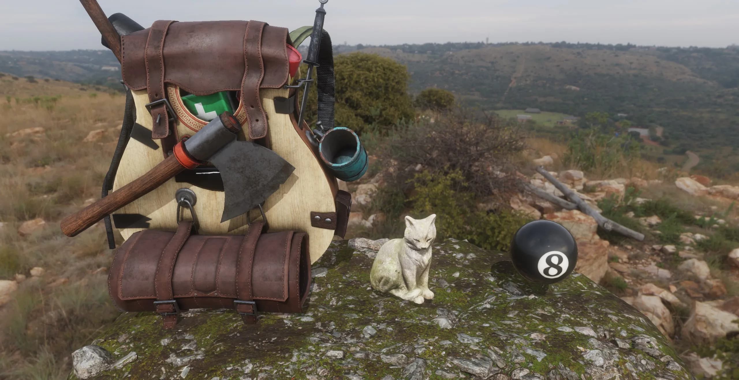
Table of Contents
Open Table of Contents
Assets
Before we talk about how things are rendered, let’s talk about how the models and textures used are loaded.
3D Models
Most of the complex stuff about 3D models loading is handled by the amazing Assimp library. Although it greatly simplifies the process, it’s still necessary to see how each 3D model format is stored. As the renderer started by using the Blinn-Phong lighting model, it was easier to use the OBJ format. The fact that everything is editable by text made it really convenient to use and edit. However, as the renderer moved to PBR, it became more and more complex to use OBJs, as the standard doesn’t define how the PBR materials should be stored, and each program/library does it its own way. Furthermore, OBJ stores the vertex data in plain text. This makes it really slow to load and parse, as a lot of memory is wasted. All of those facts made me move to a more suited format: glTF.
glTF stores the vertex data in binary format, and even has to option to store everything in binary with .glb files. obj2gltf allowed me to convert all my OBJ models to glTF, and it even has the option to merge the ambient occlusion, roughness and metallic (ARM) maps into one file.
With my glTFs in hand, I had to adapt my asset loading code.
As I still wanted to support models that have three separate textures for the ARM maps, I decided to check if the model had an ARM map.
But to my surprise, Assimp doesn’t have an option to check this, which means the only way to know is to check the texture type aiTextureType_UNKNOWN.
To make things worse, this ARM map counts as a roughness map and as a metalness.
So if you’re not careful, you might load the map three times.
But with everything I needed to know in mind, I could write my material loading function.
// The function returns a vector because I later need to see if the meshes
// that I'm loading have a material that I can handle
std::vector<std::size_t> stw::MaterialManager::LoadMaterialsFromAssimpScene(
	const aiScene* assimpScene, const std::filesystem::path& workingDirectory, TextureManager& textureManager) {
	const std::span<aiMaterial*> assimpMaterials{ assimpScene->mMaterials, assimpScene->mNumMaterials };

	std::vector<std::size_t> assimpMaterialIndicesLoaded;
	assimpMaterialIndicesLoaded.reserve(assimpMaterials.size());

	for (usize i = 0; i < assimpMaterials.size(); i++) {
		aiMaterial* material = assimpMaterials[i];
		auto diffuseCount = material->GetTextureCount(aiTextureType_DIFFUSE);
		auto baseColorCount = material->GetTextureCount(aiTextureType_BASE_COLOR);
		// ...
		auto unknownCount = material->GetTextureCount(aiTextureType_UNKNOWN);

		if ((diffuseCount > 0 || baseColorCount > 0) &&
			normalCount > 0 &&
			roughnessCount > 0 &&
			metallicCount > 0) {
			if (unknownCount == 0) {
				if (ambientCount > 0 || ambientOcclusionCount > 0) {
					LoadPbrNormal(material, workingDirectory, textureManager);
					assimpMaterialIndicesLoaded.push_back(i);
				} else {
					LoadPbrNormalNoAo(material, workingDirectory, textureManager);
					assimpMaterialIndicesLoaded.push_back(i);
				}
			} else {
				LoadPbrNormalArm(material, workingDirectory, textureManager);
				assimpMaterialIndicesLoaded.push_back(i);
			}
		} else {
			spdlog::debug("Unhandled material");
		}
	}

	return assimpMaterialIndicesLoaded;
}
Textures
Textures where way easier to handle than 3D models.
All you have to do is give a path to stb_image, get the char*, give it to OpenGL and tada!
However, this was, unfortunately, the slowest part of the asset loading code. I would often spend 20ms on Assimp’s code and my code reading Assimps data and then 2200ms on texture loading.
This is why I then decided to use another format: KTX. This format has the benefit to be readable by the GPU, which gives way better performance when loading it and giving it to the GPU. It also has the benefit of having some metadata on how the format should be read by OpenGL (such as if it’s in linear space or in SRGB). I was also able to bake the mipmaps directly inside the file and to compress it to make it even smaller than the PNG (from 33 MB to 8 MB).
To add to the list of great things of this format, the loading code was really easy to implement thanks to Khronos’ libktx.
All you have to do is load the KTX with ktxTexture_CreateFromNamedFile and then give this file to ktxTexture_GLUpload.
It will then give back to you the OpenGL id that you can use for rendering.
Scene Graph
A scene graph is a way to organise elements in a scene by having elements that are children of other elements. If the parent moves, all of its children must move in the same way.
Having already implemented a scene graph on my C# CPU rasterizer project 3D Viewer,
I had a rough idea of what I needed to do to implement it.
That said, in 3D viewer my scene graph worked by having List that contained elements that contained List etc,
but this is horrible in terms of performance, so I decided to go in another direction.
My scene graph is basically made of two vectors.
std::vector<SceneGraphElement> m_Elements{};
std::vector<SceneGraphNode> m_Nodes{};
The nodes are here to describe the tree layout. They each have an index to an element. The elements have an id to their mesh and to their material. They also have their local transform matrix and their parent’s.
struct SceneGraphElement
{
	std::size_t meshId = InvalidId;
	std::size_t materialId = InvalidId;
	glm::mat4 localTransformMatrix{ 1.0f };
	glm::mat4 parentTransformMatrix{ 1.0f };
};

struct SceneGraphNode
{
	std::size_t elementId = InvalidId;
	std::optional<std::size_t> parentId{};
	std::optional<std::size_t> childId{};
	std::optional<std::size_t> siblingId{};
};
From this you might be wondering:
Buy why do you have children and siblings?
And this is a great question! As I didn’t want to store a vector of children, because it would be on the heap and would require allocations, I went with a method that avoided this. It also keeps all of the data next to each other, and this makes the structure more cache friendly. This means that my scene graph looks something like this:

And what’s nice with this code, is that traversing the tree to draw it to the screen is not that much more complex than using some good old DFS.
// This method is private
void stw::SceneGraph::ForEachChildren(
	const stw::SceneGraphNode& startNode, const std::function<void(SceneGraphElement&)>& function) {
	if (!startNode.childId) return;

	std::vector<std::size_t> nodes;
	nodes.reserve(m_Nodes.size());
	nodes.push(startNode.childId.value());
	while (!nodes.empty()) {
		const auto currentNode = nodes.back();
		nodes.pop_back();
		auto& node = m_Nodes[currentNode];
		auto& element = m_Elements[node.elementId];
		function(element);

		if (node.childId) {
			nodes.push_back(node.childId.value());
		}

		if (node.siblingId) {
			nodes.push_back(node.siblingId.value());
		}
	}
}
But right now you might notice that if we have an element that has the same material id and mesh id, we do not profit from instancing.
Well the ForEach public method on the class is here for that.
// A custom hash function is implemented for this type
struct SceneGraphElementIndex
{
	std::size_t meshId = InvalidId;
	std::size_t materialId = InvalidId;

	bool operator==(const SceneGraphElementIndex& other) const;
};

void stw::SceneGraph::ForEach(
	const std::function<void(SceneGraphElementIndex,
	std::span<const glm::mat4>)>& function) {
	// Abseil hash map because std::unordered_map is slower
	absl::flat_hash_map<SceneGraphElementIndex, std::vector<glm::mat4>> instancingMap{};

	ForEachChildren(m_Nodes[0], [&instancingMap](SceneGraphElement& element) {
		if (element.materialId == InvalidId || element.meshId == InvalidId)
			return;

		const glm::mat4 transform =
			element.parentTransformMatrix * element.localTransformMatrix;
		const SceneGraphElementIndex index{ element.meshId, element.materialId };

		instancingMap[index].push_back(transform);
	});

	for (const auto& [elementIndex, transforms] : instancingMap) {
		function(elementIndex, transforms);
	}
}
As you can see, we first loop over the graph, and each object is added to a hash map.
This map basically has the material and mesh ids as a key.
This means that we can then draw each element with their respective transforms.
One thing I don’t like with this implementation is the std::vector as value in the hash map, as it forces to do allocations for each element in the scene.
Unfortunately, I couldn’t come up with a better way to do it.
Renderer Class
One thing that helped quite a lot in this project was having a renderer class where I could implement the different computer graphics concepts away from the “user” code (this isn’t a library, but you get what I mean).
This class contains:
- OpenGL’s “global functions” (for ex.
glClear,glFrontFace) - Light management (you can add point and directional lights to it)
- All of the other managers (MaterialManager, TextureManager, SceneGraph, …)
- The framebuffers and pipelines (also known as the shader class in LearnOpenGL)
I’m not gonna show code that’s inside this class as it’s kinda messy and the .cpp is 1409 lines long as of writing (oops 😅). But the result of this is that using it is really convenient:
void Init() {
	m_Renderer->Init(screenSize);
														// Flag to flip UVs
	result = m_Renderer->LoadModel("./data/cat_gltf/cat.gltf", true);
	if (!result.has_value())
	{
		spdlog::error("Error on model loading : {}", result.error());
	}

	auto nodeVec = result.value();
	m_CatNodeIndex = nodeVec[0];
	m_Renderer->GetSceneGraph().TranslateElement(
		m_CatNodeIndex, glm::vec3{ 0.3f, 0.4f, 0.0f });
	m_Renderer->GetSceneGraph().ScaleElement(
		m_CatNodeIndex, glm::vec3{ 4.0f, 4.0f, 4.0f });

	const PointLight p{ glm::vec3{ 5.0f, 0.0f, 4.0f }, glm::vec3{ 20.0f } };
	m_Renderer->PushPointLight(p);
}

void Update() {
	m_Renderer->Clear(GL_COLOR_BUFFER_BIT | GL_DEPTH_BUFFER_BIT);

	// As long as you don't look into Init and DrawScene, everything is fine!
	m_Renderer->DrawScene();
}

void Delete() {
	m_Renderer->Delete();
}
Materials
As you saw above, I wanted to be able to load models that have different kind of materials in the project. For example, one material could have an ambient occlusion map and another one might not. This is where my material system comes into place.
First, each material is defined as a struct that has an id of each texture is possess.
struct MaterialPbrNormalArm
{
	std::size_t baseColorMapIndex{};
	std::size_t normalMapIndex{};
	std::size_t armMapIndex{};
};
Then each material is placed in a std::variant.
I chose this class because it’s the closest thing we have in C++ to Rust’s wonderful enums.
using Material = std::variant<InvalidMaterial, MaterialPbrNormal, MaterialPbrNormalNoAo, MaterialPbrNormalArm>;This means that when I need to bind the material’s textures for the geometry pass, I can use std::visit
which will call the correct lambda for the current material.
using GBufferPipelinesArray =
	std::array<std::reference_wrapper<stw::Pipeline>, MaterialCount>;

void stw::BindMaterialForGBuffer(
	const stw::Material& materialVariant,
	stw::TextureManager& textureManager,
	const GBufferPipelinesArray& gBufferPipelines
)
{
	// Other lambdas

	const auto pbrNormalArm = [&textureManager, &gBufferPipelines](const MaterialPbrNormalArm& material) {
		const Pipeline& pipeline = gBufferPipelines[2];
		pipeline.Bind();
		// Bind each texture...
	};

	constexpr auto invalid = [](const InvalidMaterial&) {
		spdlog::error("Invalid material... {} {}", __FILE__, __LINE__);
	};

	std::visit(
		Overloaded{ invalid, pbrNormal, pbrNormalNoAo, pbrNormalArm },
		materialVariant
	);
}
Shadow Maps
Shadow Maps in View-space
I won’t explain how I implemented shadow maps, as this fairly well explained in LearnOpenGL. I will however mention one thing: shadow maps with view-space fragment position. In LearnOpenGL, to implement SSAO, the author explains that view-space fragment positons are required, but every other chapter on the website consider them to be in world-space. This is quite frustrating, because the change from one to the other is not trivial.
For point lights, the change is quite simple. You just use the negative of the fragment’s position as the vector that points to the view and pass the light’s position transformed by the view matrix.
vec3 viewDir = normalize(-fragPos);And if we didn’t have shadow maps, it would be the same for the directional light.
Only the direction vector would have to be transformed by the view matrix.
But there is this lightViewProjMatrix that is responsible for transforming the fragment’s position from world-space to the light’s view-space.
Now ideally we would want this matrix to make the fragment go from the camera’s view-space to the light’s view-space.
And fortunately, it’s possible! You just have to multiply the lightViewProjMatrix by the inverse of the camera view matrix when you create it.
In summary:
glm::vec4 lightViewProjMatrix =
	lightProjection * lightView * glm::inverse(cameraView);
But now we have a problem in the depth pass that renders the light’s shadow buffer, since it’s supposed to multiply the vertices by the model matrix and the light view projection matrix. I guess the smart way to do it would be to create two matrices, one for the shadow pass and one for the directional light pass, but I choose to just multiply the light view projection matrix by the camera view matrix to invert the inverse (what?).
#version 430

layout (location = 0) in vec3 aPos;
layout (location = 4) in mat4 modelMatrix;

uniform mat4 lightViewProjMatrix;

layout (std140, binding = 0) uniform Matrices
{
	mat4 projection;
	mat4 view;
};

void main()
{
	gl_Position = lightViewProjMatrix * view *  modelMatrix * vec4(aPos, 1.0);
}
Cascaded Shadow Maps
Cascaded shadow maps are conceptually quite simple to implement, the hardest part is having a light that englobes the view frustum (or part of it as we will see).
My implementation is a mix of multiple ones I found on the internet, but the one that helped the most is from OGL.
One thing I really struggled with, is having weird shadows although the math seemed correct. The problem almost always came from the light’s view frustum that wasn’t of a correct size. To fix this, after computing the part of the camera view frustum I wanted to see for this map, I added some margin to the size of the light view frustum.
// Compute max and mix like in OGL's tutorial

f32 midLenX = (maxX - minX) / 2.0f;
f32 midLenY = (maxY - minY) / 2.0f;
f32 midLenZ = (maxZ - minZ) / 2.0f;

const f32 midX = minX + midLenX;
const f32 midY = minY + midLenY;
const f32 midZ = minZ + midLenZ;

constexpr f32 zMultiplier = 5.0f;
constexpr f32 xyMargin = 1.1f;
midLenX *= xyMargin;
midLenY *= xyMargin;
midLenZ *= zMultiplier;

const glm::vec3 minLightProj{ midX - midLenX, midY - midLenY, midZ - midLenZ };
const glm::vec3 maxLightProj{ midX + midLenX, midY + midLenY, midZ + midLenZ };
zMultiplier and xyMargin are two constants I changed depending on the artifacts I would get when modifying the engine.
The steps of a deferred rendered frame
So now that we know some of the secrets that make up the engine, let’s look at what a frame is made out of.
The first thing that’s done is the geometry pass all of the informations that the future passes are gonna need into one framebuffer with three color attachments.
The first attachment has the fragments positions in view-space on the RGB channels and the ambient occlusion factor in the alpha.
Then in the second attachment, the normals in view-space and the roughness are stored.
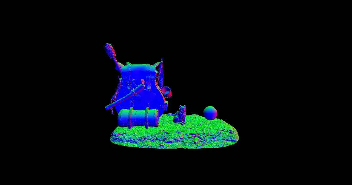
And in the third attachment, we have the base color and the metallic.

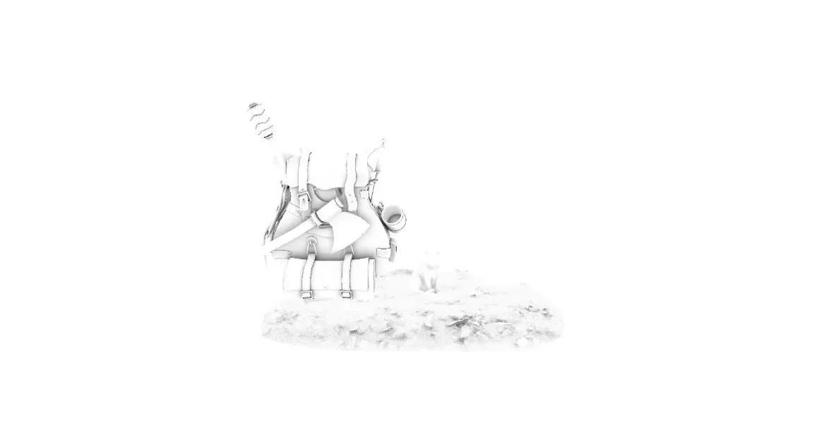
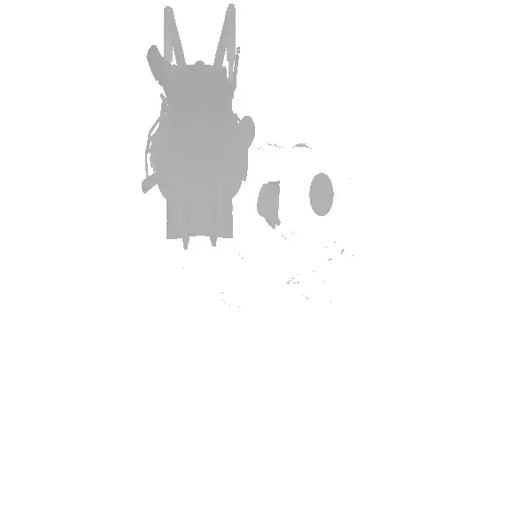
After this pass, we take the fragments in view-space and use them to compute the SSAO. A blur effect is then applied to smooth out the noise.

Then, the four levels of the cascaded shadow maps are rendered. (I’ll only show two of them.)
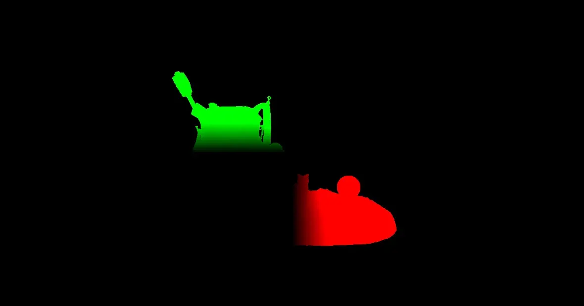
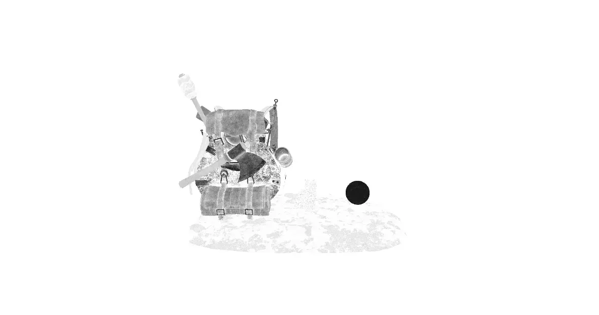
After this, we can start to render the lights. For this, we enable blending and call three pipelines:
- Ambient lighting (IBL)
- Directional light (with shadow)
- Point lights
The ambient lighting and directional light are rendered using a quad that’s the size of the screen, because they apply to every object. Then, the point lights are rendered by rendering a sphere that has the same position and radius of the light. This allows to only update the pixels impacted by the light and saves on performance.
The ambient lighting looks like this:
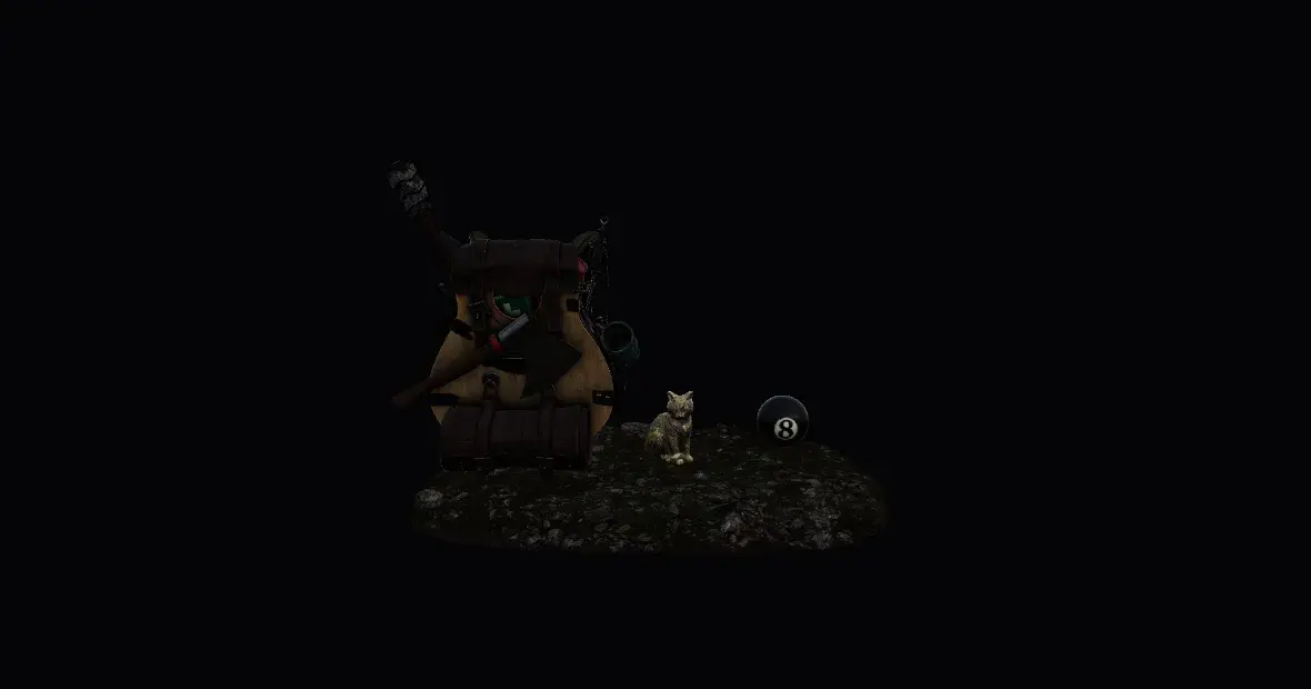
Then the point light (yes it’s very similar):

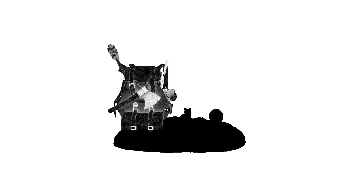
And finally the directional light:
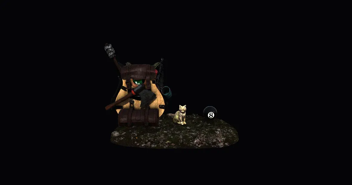
Now that the light computation is done, spheres that are the color of the lights are rendered on top of the attachment and the skybox is drawn.
Then bloom is rendered.
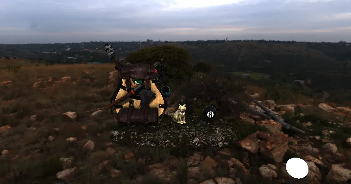
And now we can mix the bloom with the previous framebuffer and apply some HDR tone mapping and gamma correction. (In my case I use Narkowicz ACES).
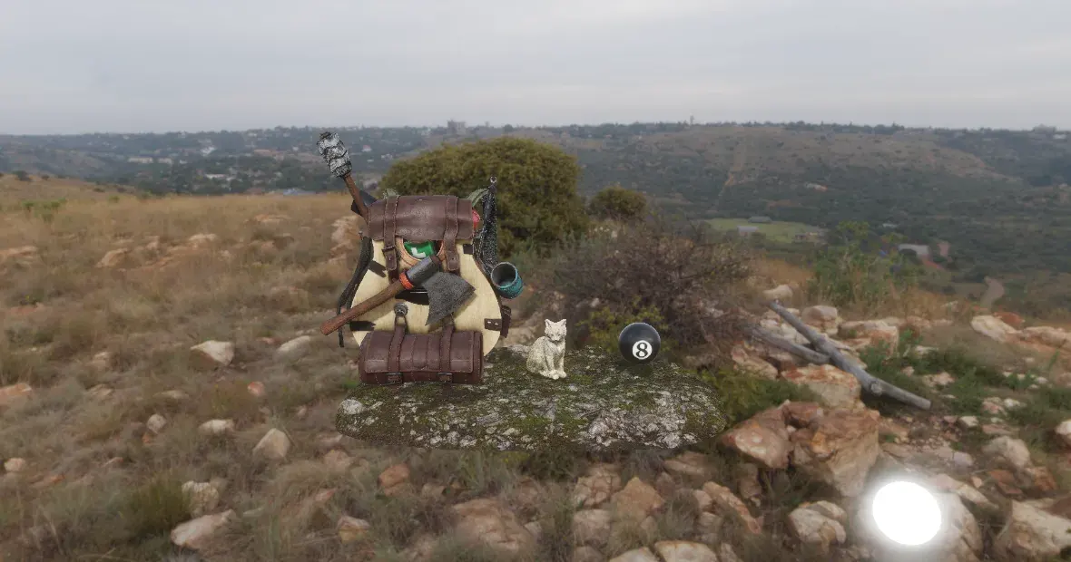
Et voilà! It took a lot of effort, but we have our final image.
Conclusion
I’m really proud of what I’ve done. Computer graphics is the domain where I want to work and this project taught me a lot. I think I put in a lot of work, and the final result shows it.
That being said, there are still some things I could improve. Such as:
- Structure of the code (especially renderer.cpp)
- Add Frustum Culling
- Add a bit of multi-threading somewhere
- Do some benchmarks and analyze the code with tracy to optimize it a bit (this one is just for fun)
You can find the code of this project on my GitHub.
In the longer term, I really want to explore other graphics API using other programming languages.
Right now my goals are:
- Direct3D 11: Odin
- Direct3D 12: Zig
- Vulkan: Rust
I hope I’ll be able to work on these projects and maybe write a blogpost about it!
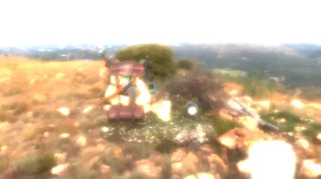
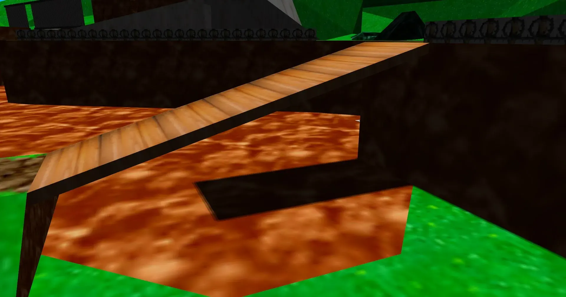
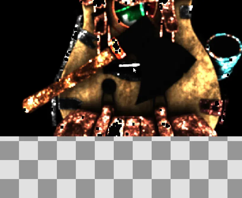
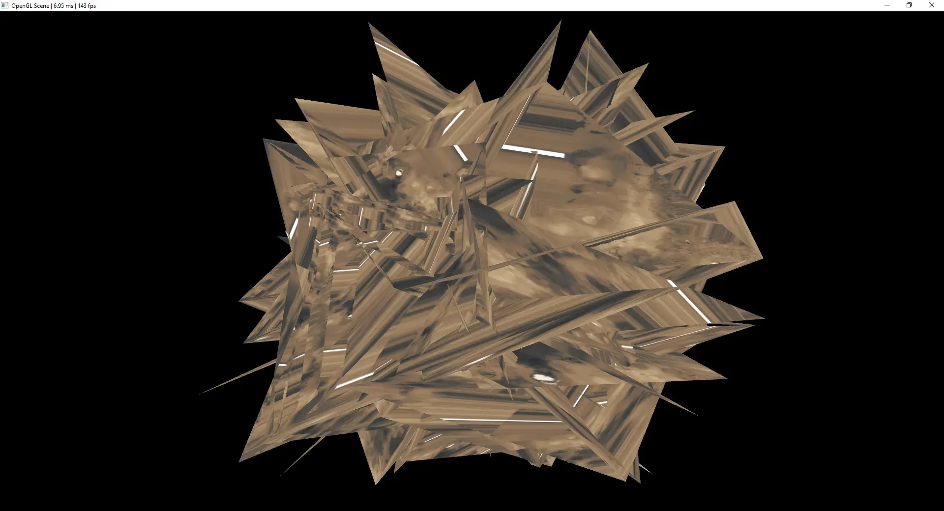
now some bonus funny visual bugs
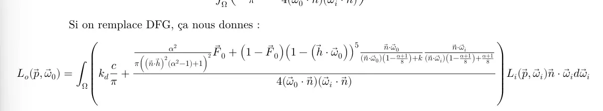
and the full IBL developed integral because why not